How to Deal with Fuzziness?

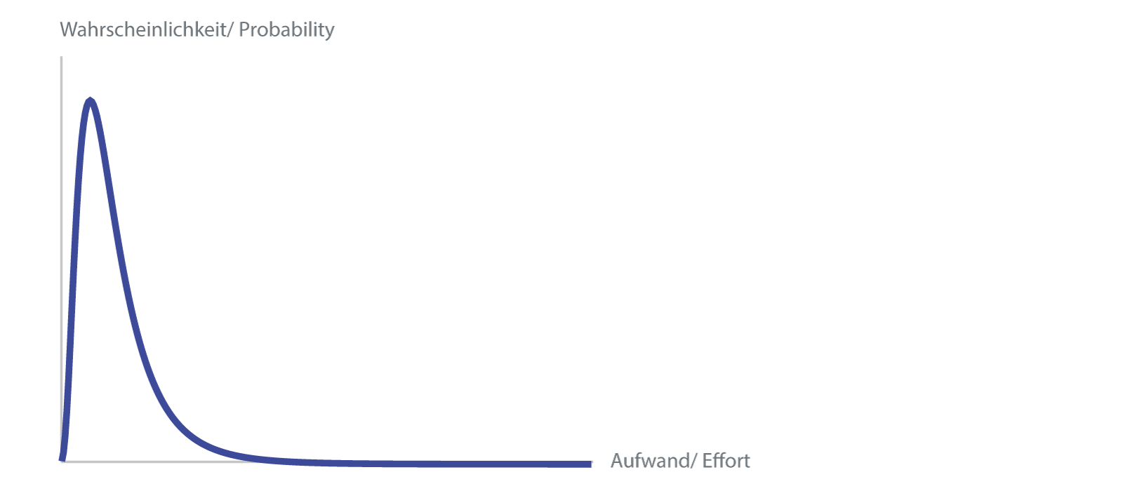
Probability Distribution (lognormal)

Now, of course, one does not want to discuss the exact curve for each work package, so one assumes certain curve shapes as a model that can be described with a few parameters.

In the next sections, different approaches to this will be discussed.

• Three-Point Estimation: The exact way
• Two-Point Estimation: How to make it easier, with optimism compensation
• Lognormal Distribution: An asymmetric distribution
• The 90% Confidence Interval: How much risk would you like to take?
• Central Limit Theorem: How many inaccurate estimates lead to the exact result

Experience has shown that there is often a tendency to optimism among estimators as tasks and difficulties are forgotten. Therefore, Barry W. Boehm (in [R. D. Stutzke: „Estimating Software Intensive Systems”, 2005, ISBN 0-201-70312-2]) has given greater weight to the worst case value G in the 3-point effort estimation by shifting a weight from the normal case to the worst case:

Two-Point Estimation

Indirectly, [W. Reiter: „Die nackte Wahrheit über Projektmanagement”, 2003 ISBN 3-280-05018-9] chose a different approach by shifting the weight from the optimal case K to the worst case G in his formula:

In addition to the optimism correction, this two-point effort estimation has the advantage that one of three estimation values and thus a part of the estimation effort can be saved.

Optimism? Really?

In [N. N. Taleb: „Antifragile”, 2012 ISBN 1-400-06782-0], in the chapter „Why planes don't arrive early” there is another, philosophical explanation for the fact that projects always tend to be underestimated. One rarely plans too much, the more complex the project, the activity, the more is forgotten. Since the time spent on such forgotten activities is always positive, the total effort can only increase, never decrease.

Justification of the two-point effort estimation with the normal distribution

If the whole PERT story is too empirical for you, you can also justify the above formula with the normal distribution, as in [W. Reiter: «Die nackte Wahrheit über Projektmanagement», 2003 ISBN 3-280-05018-9], according to the following illustration:

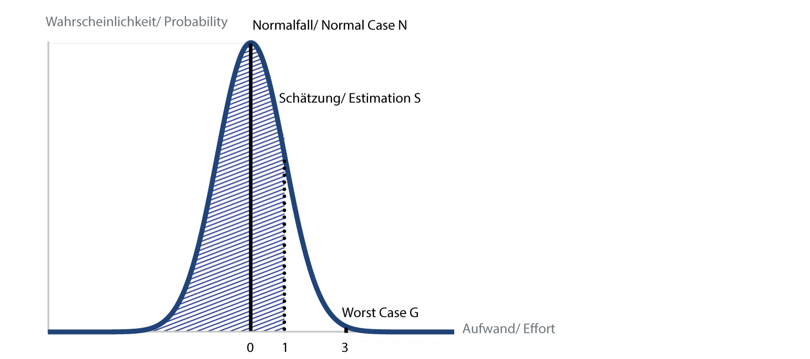
Two-Point Estimation

Normal distribution with estimate and the 84% area marked

Marked are the normal case N and the worst case G. Now we specify that we want to be below the worst case G for 99.9% of the cases. This allows us to fit a normal distribution („Gaussian curve/ Bell curve”), where the normal case corresponds to the peak value, i.e. the most frequent case, the worst case corresponds to a deviation of three standard deviations („3 sigma”), the small remainder above then corresponds to a probability of 0.1 %.

We further specify that we would like our estimate to be below the estimated value in 84 % of the cases. This corresponds to a standard deviation („1 sigma”), which is on the third of the way between normal and worst case. Written out as a formula:

So the same result as above. What is unattractive about this type of reasoning is the fact that the normal distribution also allows for negative effort. While this would sometimes be nice for project managers, I have not heard of anyone who has finished a job before they started.

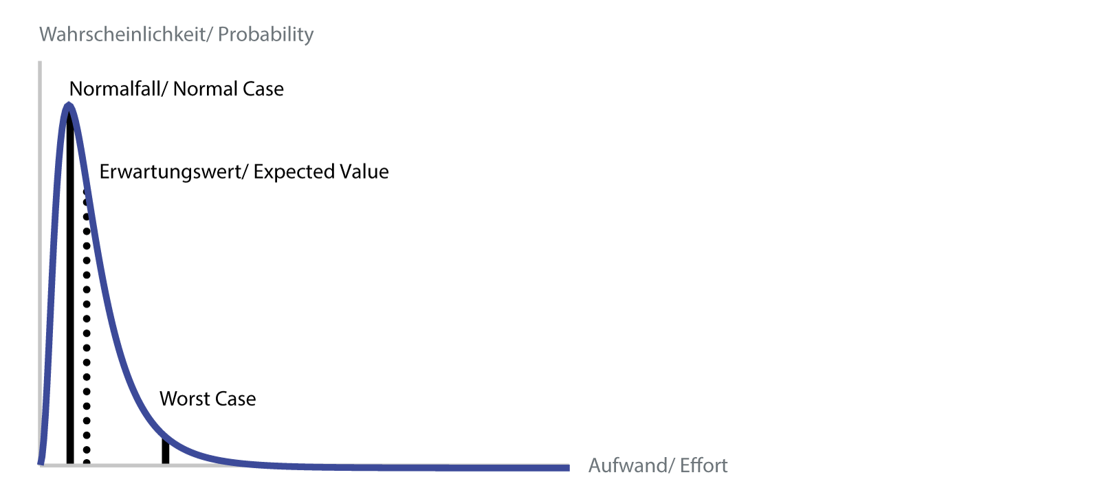
Lognormal distribution with estimated values

As a model for our purposes the lognormal distribution is suitable, because on the one hand it covers a range of values above zero and on the other hand it can be completely characterized by two parameters, in our case by the normal value and the worst case. The normal case is defined as the case where the probability is greatest, that is, the peak value. The worst case value can again be chosen at 99.9%. We ourselves use 95%, this also results in a certain correction of the optimism of the estimators.

The expected value, i.e. the value that one would most likely expect, is the mean value, which in this distribution, unlike the normal distribution, does not coincide with the peak value. The big disadvantage of the lognormal distribution is that one has to use numerical methods or Monte Carlo simulations to calculate sums and products. A simple implementation as a spreadsheet is not possible.

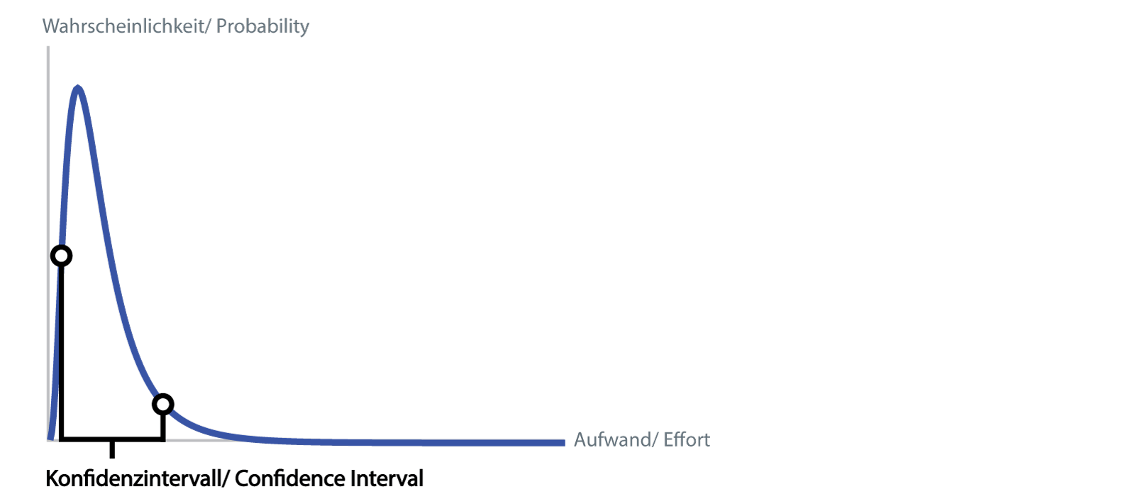
Confidence Interval

In other words, the probability is 5% that the effort is below the lower threshold, 5% that it is above the upper threshold. The width of the confidence interval also provides a good measure of the risk of the project: an interval of 2000 to 6000 hours indicates a riskier project than one of 3000 to 5000 hours.

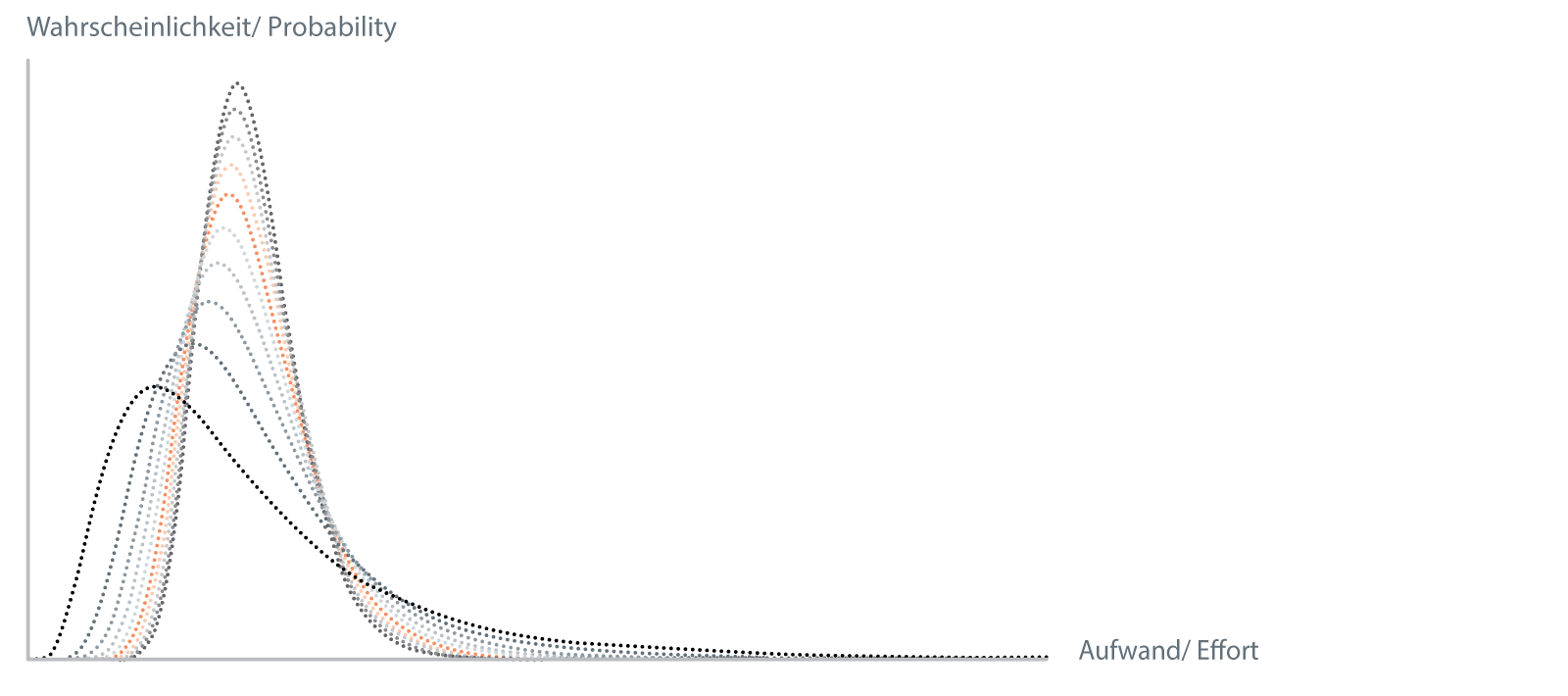
Summation of lognormal distributed random variables

In the above image, you can see how a lognormal distribution is convolved with itself ten times, which corresponds to the addition of the underlying random variables. The resulting distribution has been scaled by the number of convolutions in each case, so you can see how the shape of the distribution changes.

Immediately notice how the resulting distribution gets narrower at each step. This is the central limit theorem of probability theory, which states, among other things, that under various conditions the distribution function of summed random variables becomes narrower and narrower.

For us, the most important of these conditions is independence, i.e. that the various estimation elements must not influence each other. For project management, this is certainly wrong, since each estimated package, if it takes longer, for example, will increase the total duration of the project and thus increase the effort required to manage the project. This general problem can be addressed by estimating such dependent packages (e.g., system testing and bug fixing) only at the end, when the effort for the whole rest of the project is already known.